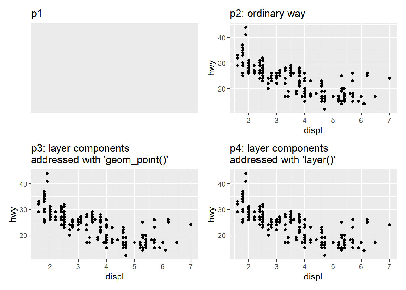
geom_point() is a shortcut. Behind the scenes it calls the layer() function to create a new layer. … It’s useful to understand the layer() function so you have a better mental model of the layer object. But you’ll rarely use the full layer() call because it’s so verbose (冗长的).
Each layer (of ggplot2) can come from a different dataset and have a different aesthetic mapping, making it possible to create sophisticated plots that display data from multiple sources.
… the details of a layer … five components: data, the aesthetic mappings, the geom, stat, and position adjustment.
Gradient scales provide a robust method for creating any colour scheme you like. All you need to do is specify two or more reference colors, and ggplot2 will interpolate linearly between them …:
scale_fill_gradient() produces a two-colour gradient scale_fill_gradient2() produces a three-color gradient with specified midpoint. scale_fill_gradientn() produces an n-color gradient
Internally, ggplot2 handles discrete scales by mapping each category to an integer value and then drawing the geom at the corresponding coordinate location.
ggplot2 specifies the size in millimeters (mm), rather than the usual points (pts). The reason for this choice is that it makes it the units for font sizes consistent with how other sizes are specified in ggplot2. (There are 72.27 pts in a inch)
There are two groups of graphics devices (GDs): screen devices such as windows() (for Windows), quartz() (for Macs), X11() (mostly for Linux) and RStudioGD() (within RStudio) draw the plot to the screen, whereas file devices such as png() and pdf() write the plot to a file.
ggraph builds on top of tidygraph and ggplot2 to allow a complete and familiar grammar of graphics for network data. … works with another data type that is fundamentally different from tabular data. … concerned with showing the network topology more than relations between two variables. Layouts are algorithms that use the network structure to calculate (often arbitrary) x and y values for each node … for visualization purposes.
Perhaps the simplest approach to draw maps is to use geom_polygon() to draw doundaries for different regions.
Vector data for maps are typically encoded using the “simple features” standard produced by the Open Geospatial Consortium.
… in which (i.e. simple features) geographical entities are specified in terms of a set of lines, points and polygons, rasters take the form of images … For example … GeoTIFF, which is a regular TIFF file with additional metadata supplied.
The grid package provides the underlying graphics system upon which ggplot2 is built. It’s one of two quite different drawing systems that are included in base R: base graphics and grid.
If you kill Americans, if you threaten Americans anywhere on earth, well will hunt you down without apology and without hesitation, and we will kill you.